Classifying the “German Credit” Dataset
This dataset has two classes (these would be considered labels in Machine Learning terms) to describe the worthiness of a personal loan: “Good” or “Bad”. There are predictors related to attributes, such as: checking account status, duration, credit history, purpose of the loan, amount of the loan, savings accounts or bonds, employment duration, installment rate in percentage of disposable income, personal information, other debtors/guarantors, residence duration, property, age, other installment plans, housing, number of existing credits, job information, number of people being liable to provide maintenance for, telephone, and foreign worker status.
Many of these predictors are discrete and have been expanded into several 0/1 indicator variables (a.k.a. they have been one-hot-encoded).
This dataset has been kindly provided by Professor Dr. Hans Hofmann of the University of Hamburg, and can also be found on the UCI Machine Learning Repository.
Building a decision tree
import pandas as pd
from sklearn.tree import DecisionTreeClassifier
from sklearn.metrics import classification_report
from sklearn.model_selection import train_test_split
from sklearn.model_selection import GridSearchCV

from sklearn.pipeline import Pipeline
from sklearn.preprocessing import StandardScaler
from sklearn.compose import ColumnTransformer

from sklearn.metrics import accuracy_score
from sklearn.metrics import balanced_accuracy_score
from sklearn.metrics import ConfusionMatrixDisplay

import seaborn as sns
import matplotlib.pyplot as plt

import warnings
warnings.filterwarnings('ignore')
df = pd.read_csv('./GermanCredit.csv.zip')
df.head()
Console output (1/1):
.dataframe tbody tr th {
    vertical-align: top;
}

.dataframe thead th {
    text-align: right;
}
df.info()
Console output (1/1):
<class 'pandas.core.frame.DataFrame'>
RangeIndex: 1000 entries, 0 to 999
Data columns (total 62 columns):
 #   Column                                  Non-Null Count  Dtype
---  ------                                  --------------  -----
 0   Duration                                1000 non-null   int64
 1   Amount                                  1000 non-null   int64
 2   InstallmentRatePercentage               1000 non-null   int64
 3   ResidenceDuration                       1000 non-null   int64
 4   Age                                     1000 non-null   int64
 5   NumberExistingCredits                   1000 non-null   int64
 6   NumberPeopleMaintenance                 1000 non-null   int64
 7   Telephone                               1000 non-null   int64
 8   ForeignWorker                           1000 non-null   int64
 9   Class                                   1000 non-null   object
 10  CheckingAccountStatus.lt.0              1000 non-null   int64
 11  CheckingAccountStatus.0.to.200          1000 non-null   int64
 12  CheckingAccountStatus.gt.200            1000 non-null   int64
 13  CheckingAccountStatus.none              1000 non-null   int64
 14  CreditHistory.NoCredit.AllPaid          1000 non-null   int64
 15  CreditHistory.ThisBank.AllPaid          1000 non-null   int64
 16  CreditHistory.PaidDuly                  1000 non-null   int64
 17  CreditHistory.Delay                     1000 non-null   int64
 18  CreditHistory.Critical                  1000 non-null   int64
 19  Purpose.NewCar                          1000 non-null   int64
 20  Purpose.UsedCar                         1000 non-null   int64
 21  Purpose.Furniture.Equipment             1000 non-null   int64
 22  Purpose.Radio.Television                1000 non-null   int64
 23  Purpose.DomesticAppliance               1000 non-null   int64
 24  Purpose.Repairs                         1000 non-null   int64
 25  Purpose.Education                       1000 non-null   int64
 26  Purpose.Vacation                        1000 non-null   int64
 27  Purpose.Retraining                      1000 non-null   int64
 28  Purpose.Business                        1000 non-null   int64
 29  Purpose.Other                           1000 non-null   int64
 30  SavingsAccountBonds.lt.100              1000 non-null   int64
 31  SavingsAccountBonds.100.to.500          1000 non-null   int64
 32  SavingsAccountBonds.500.to.1000         1000 non-null   int64
 33  SavingsAccountBonds.gt.1000             1000 non-null   int64
 34  SavingsAccountBonds.Unknown             1000 non-null   int64
 35  EmploymentDuration.lt.1                 1000 non-null   int64
 36  EmploymentDuration.1.to.4               1000 non-null   int64
 37  EmploymentDuration.4.to.7               1000 non-null   int64
 38  EmploymentDuration.gt.7                 1000 non-null   int64
 39  EmploymentDuration.Unemployed           1000 non-null   int64
 40  Personal.Male.Divorced.Seperated        1000 non-null   int64
 41  Personal.Female.NotSingle               1000 non-null   int64
 42  Personal.Male.Single                    1000 non-null   int64
 43  Personal.Male.Married.Widowed           1000 non-null   int64
 44  Personal.Female.Single                  1000 non-null   int64
 45  OtherDebtorsGuarantors.None             1000 non-null   int64
 46  OtherDebtorsGuarantors.CoApplicant      1000 non-null   int64
 47  OtherDebtorsGuarantors.Guarantor        1000 non-null   int64
 48  Property.RealEstate                     1000 non-null   int64
 49  Property.Insurance                      1000 non-null   int64
 50  Property.CarOther                       1000 non-null   int64
 51  Property.Unknown                        1000 non-null   int64
 52  OtherInstallmentPlans.Bank              1000 non-null   int64
 53  OtherInstallmentPlans.Stores            1000 non-null   int64
 54  OtherInstallmentPlans.None              1000 non-null   int64
 55  Housing.Rent                            1000 non-null   int64
 56  Housing.Own                             1000 non-null   int64
 57  Housing.ForFree                         1000 non-null   int64
 58  Job.UnemployedUnskilled                 1000 non-null   int64
 59  Job.UnskilledResident                   1000 non-null   int64
 60  Job.SkilledEmployee                     1000 non-null   int64
 61  Job.Management.SelfEmp.HighlyQualified  1000 non-null   int64
dtypes: int64(61), object(1)
memory usage: 484.5+ KB
df.describe()
Console output (1/1):
.dataframe tbody tr th {
    vertical-align: top;
}

.dataframe thead th {
    text-align: right;
}
Mapping classes
Good -> 1
Bad -> 0
df['Class'] = df['Class'].map({"Good":1,"Bad":0})
df['Class'].value_counts().plot(kind='bar')
plt.grid(True)
plt.title("Number of times 'Good' (1) and 'Bad' (0) appeared in dataset")
plt.show()
Console output (1/1):
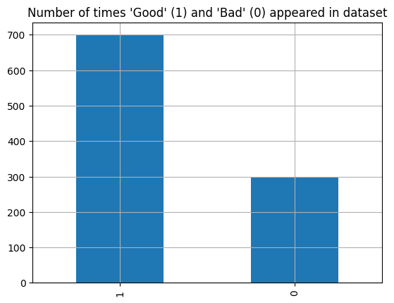
Observations
There is imbalance in the target variable, namely, there are over twice as many data points labelled as “Good” as there are points labelled as “Bad”.
Plotting the confusion matrix
def classify_grid_search_cv_tuning(model, parameters, X_train, X_test, y_train, y_test, n_folds = 5, scoring='accuracy'):
"""
This function tunes GridSearchCV model
Parameters:
----------
model
parameters
X_train
X_test
y_train
y_test
n_folds
scoring
Returns:
--------
best_model
best_score
"""
# Set up and fit model
tune_model = GridSearchCV(model, param_grid=parameters, cv=n_folds, scoring=scoring)
tune_model.fit(X_train, y_train)
best_model = tune_model.best_estimator_
best_score = tune_model.best_score_
y_pred = best_model.predict(X_test)
# Printing results
print("Best parameters:", tune_model.best_params_)
print("Cross-validated accuracy score on training data: {:0.4f}".format(tune_model.best_score_))
print()
print(classification_report(y_test, y_pred))
return best_model, best_score
# Use function
# Set dependend and independent variables
X = df.drop('Class', axis=1)
y = df['Class']
# Split data into training and testing data
X_train, X_test, y_train, y_test = train_test_split(X, y, train_size=0.8, random_state=1)
# Set pipeline
numeric_transformer = Pipeline(
steps=[("scaler", StandardScaler())]
)
preprocessor = ColumnTransformer(
transformers=[
("num", numeric_transformer, X.columns),
]
)
model_classifier = Pipeline(
steps=[("preprocessor", preprocessor), ("DecisionTree", DecisionTreeClassifier(min_samples_leaf=2, random_state=1))] #colsample by tree, n estimators, max depth
)
# Set initial model
model_classifier.fit(X_train, y_train)
y_pred = model_classifier.predict(X_test)
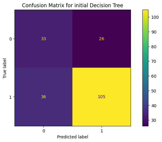
fig, ax = plt.subplots(figsize=(10, 5))
ConfusionMatrixDisplay.from_predictions(y_test, y_pred, ax=ax)
_ = ax.set_title(
f"Confusion Matrix for initial Decision Tree"
)
plt.show()
Console output (1/1):
Improving model performance with hyper parameter tuning
from imblearn.pipeline import make_pipeline
from imblearn.over_sampling import SMOTE

# Set parameters
params = {'criterion': [ 'entropy'],
           'splitter': ['random'],
           'max_depth': range(5, 25),
           'max_features': range(30,60)}

decision_tree_smote_pipeline = make_pipeline(
                    preprocessor,
                    SMOTE(random_state=42),
                      DecisionTreeClassifier(min_samples_leaf=2, random_state=1)
                     )

new_params = {'decisiontreeclassifier__' + key: params[key] for key in params}
best_dtc, dtc_score = classify_grid_search_cv_tuning(decision_tree_smote_pipeline, new_params, X_train, X_test, y_train, y_test, n_folds=5, scoring='f1_weighted')
Console output (1/1):
Best parameters: {'decisiontreeclassifier__criterion': 'entropy', 'decisiontreeclassifier__max_depth': 11, 'decisiontreeclassifier__max_features': 44, 'decisiontreeclassifier__splitter': 'random'}
Cross-validated accuracy score on training data: 0.7356

              precision    recall  f1-score   support

           0       0.52      0.51      0.51        59
           1       0.80      0.80      0.80       141

    accuracy                           0.71       200
   macro avg       0.66      0.65      0.66       200
weighted avg       0.71      0.71      0.71       200
best_dtc.fit(X_train, y_train)
y_pred = best_dtc.predict(X_test)
score_train = best_dtc.score(X_train, y_train)
score_test = best_dtc.score(X_test, y_test)
# Print scores
print('score for training set', score_train, 'score for testing set', score_test)
balanced_accuracy = balanced_accuracy_score(y_test, y_pred)
print("Balanced accuracy score", balanced_accuracy)
# Print classification report
print(classification_report(y_test, y_pred))
# Plot confusion matrix
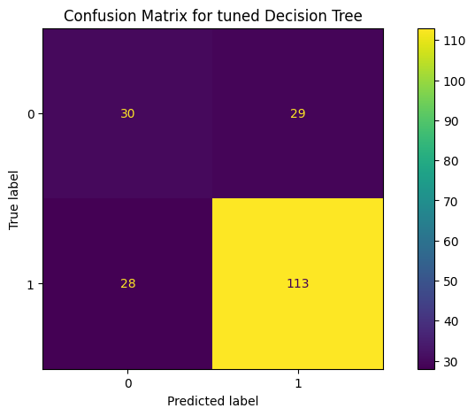
fig, ax = plt.subplots(figsize=(10, 5))
ConfusionMatrixDisplay.from_predictions(y_test, y_pred, ax=ax)
_ = ax.set_title(
f"Confusion Matrix for tuned Decision Tree"
)
plt.show()
Console output (1/2):
score for training set 0.87625 score for testing set 0.715
Balanced accuracy score 0.6549465079937493
              precision    recall  f1-score   support

           0       0.52      0.51      0.51        59
           1       0.80      0.80      0.80       141

    accuracy                           0.71       200
   macro avg       0.66      0.65      0.66       200
weighted avg       0.71      0.71      0.71       200
Console output (2/2):
Random forest
from sklearn.ensemble import RandomForestClassifier
params = [{}] # Default parameters

random_forest_smote_pipeline = make_pipeline(
                    preprocessor,
                    SMOTE(random_state=42),
                       RandomForestClassifier(random_state=1)

                     )

rforest_best,rforest_score = classify_grid_search_cv_tuning(random_forest_smote_pipeline, params, X_train, X_test, y_train, y_test, n_folds=5, scoring='f1_weighted');
Console output (1/1):
Best parameters: {}
Cross-validated accuracy score on training data: 0.7526

              precision    recall  f1-score   support

           0       0.68      0.46      0.55        59
           1       0.80      0.91      0.85       141

    accuracy                           0.78       200
   macro avg       0.74      0.68      0.70       200
weighted avg       0.76      0.78      0.76       200
rforest_best.fit(X_train, y_train)
y_pred = rforest_best.predict(X_test)
score_train = rforest_best.score(X_train, y_train)
score_test = rforest_best.score(X_test, y_test)
print('score for training set', score_train, 'score for testing set', score_test)
balanced_accuracy = balanced_accuracy_score(y_test, y_pred)
print("Balanced accuracy score", balanced_accuracy)
fig, ax = plt.subplots(figsize=(10, 5))
ConfusionMatrixDisplay.from_predictions(y_test, y_pred, ax=ax)
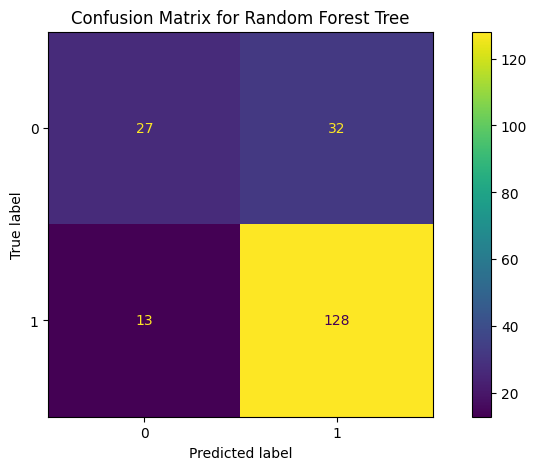
_ = ax.set_title(
f"Confusion Matrix for Random Forest Tree"
)
plt.show()
Console output (1/2):
score for training set 1.0 score for testing set 0.775
Balanced accuracy score 0.6827142685418921
Console output (2/2):
Computing feature importance
import numpy as np
importances = rforest_best._final_estimator.feature_importances_
std = np.std([tree.feature_importances_ for tree in rforest_best._final_estimator.estimators_], axis=0)

df_importances = pd.DataFrame([importances, std], index=['importances', 'std'], columns=list(X_train.columns))
df_importances = df_importances.transpose()
df_importances.sort_values('importances', ascending=False, inplace=True)
# Plot the feature importances of the forest
plt.figure(figsize=(10, 5))
plt.title("Feature importances")
plt.bar(df_importances.index, df_importances['importances'], color="r", yerr=df_importances['std'], align="center")
plt.xticks(rotation=90)
plt.xlim([-1, df_importances.shape[0]])
plt.show()
Console output (1/1):
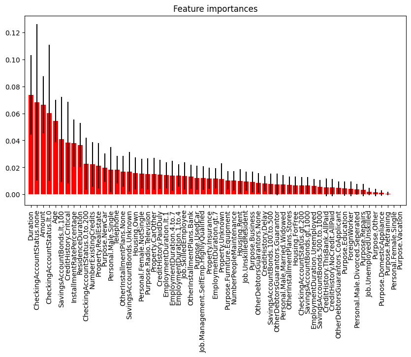
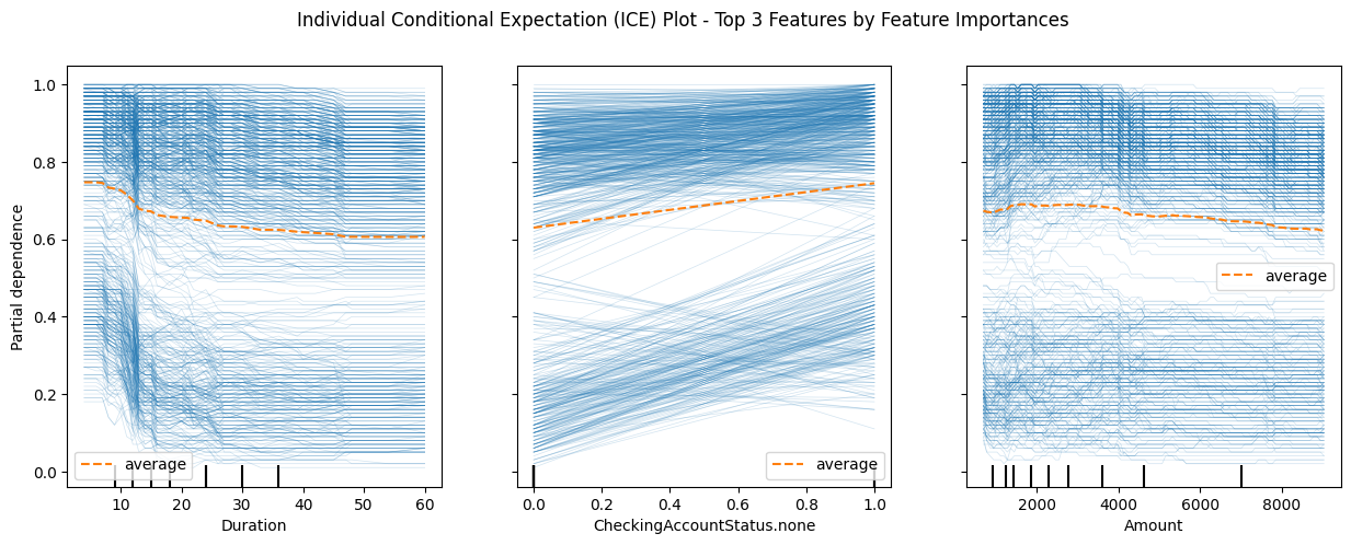
In this particular example, the top five most important features (in descending order) are:
- Duration
- CheckingAccountStatus.none
- Amount
- CheckingAccountStatus.lt.0
- Age
These features have importance scores ranging from 0.073 to 0.054, and their standard deviations suggest that the model is fairly certain about their importance rankings.
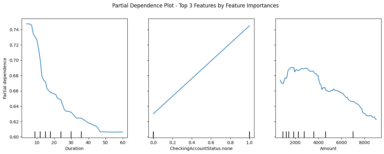
Computing Partial Dependence Plot
# compute partial dependence plot
from sklearn.inspection import PartialDependenceDisplay
PartialDependenceDisplay.from_estimator(rforest_best, X_train, ["Duration", "CheckingAccountStatus.none", "Amount"], kind='average')
cf = plt.gcf()
cf.suptitle("Partial Dependence Plot - Top 3 Features by Feature Importances");
cf.set_size_inches(15, 5)
Console output (1/1):
PartialDependenceDisplay.from_estimator(rforest_best, X_train, ["Duration", "CheckingAccountStatus.none", "Amount"], kind='both',
                                        ice_lines_kw={"color": "tab:blue", "alpha": 0.2, "linewidth": 0.5},
                                        pd_line_kw={"color": "tab:orange", "linestyle": "--"}
                                       )
cf = plt.gcf()
cf.suptitle("Individual Conditional Expectation (ICE) Plot - Top 3 Features by Feature Importances");
cf.set_size_inches(15, 5)
Console output (1/1):