Movie recommender system
Data
The data used here has been compiled from various movie datasets like Netflix and IMDb.
- Filename:
movie_titles.csv:
MovieID: MovieID does not correspond to actual Netflix movie ids or IMDB movie idsYearOfRelease: YearOfRelease can range from 1890 to 2005 and may correspond to the release of corresponding DVD, not necessarily its theaterical releaseTitle: Title is the Netflix movie title and may not correspond to titles used on other sites. Titles are in English
- Combined User-Ratings Dataset Description -
combined_data.csv:
-
The first line of the contains the movie id followed by a colon.
-
Each subsequent line in the file corresponds to a rating from a customer and its date in the following format:
- MovieIDs range from 1 to 17770 sequentially.
- CustomerIDs range from 1 to 2649429, with gaps. There are 480189 users.
- Ratings are on a five star (integral) scale from 1 to 5.
- Dates have the format YYYY-MM-DD.
- Filename:
movies_metadata.csv
The main Movies Metadata file. Contains information on 45,000 movies featured in the Full MovieLens dataset. Features include posters, backdrops, budget, revenue, release dates, languages, production countries and companies.
import pandas as pd
import matplotlib.pyplot as plt
import seaborn as sns

# To compute similarities between vectors
from sklearn.metrics import mean_squared_error
from sklearn.metrics.pairwise import cosine_similarity
from sklearn.feature_extraction.text import TfidfVectorizer

from collections import deque
def slice_movie_ratings_data(df):
    """
    Slices the movie ratings data into separate dataframes for each movie.

    Args:
        df (pd.DataFrame): A DataFrame containing the movie ratings data.

    Returns:
        list: A list of DataFrames containing the movie ratings data for each movie.
    """
    tmp_movies = df[df['Rating'].isna()]['User'].reset_index()
    movie_indices = [[index, int(movie[:-1])] for index, movie in tmp_movies.values]

    shifted_movie_indices = deque(movie_indices)
    shifted_movie_indices.rotate(-1)

    user_data = []

    for [df_id_1, movie_id], [df_id_2, next_movie_id] in zip(movie_indices, shifted_movie_indices):
        if df_id_1 < df_id_2:
            tmp_df = df.loc[df_id_1+1:df_id_2-1].copy()
        else:
            tmp_df = df.loc[df_id_1+1:].copy()
        tmp_df['Movie'] = movie_id
        user_data.append(tmp_df)

    return user_data


def combine_movie_ratings_data(dataframes):
    """
    Combines the movie ratings data for each movie into a single DataFrame.

    Args:
        dataframes (list): A list of DataFrames containing the movie ratings data for each movie.

    Returns:
        pd.DataFrame: A DataFrame containing the combined movie ratings data.
    """
    df = pd.concat(dataframes)
    return df
Load the movie metadataset
# !pip install gdown
!gdown "https://drive.google.com/uc?export=download&id=1z0O0fXuofdsbpL8fkCVgjeIwFP_LxGX2" -O data/combined_data.csv.zip
movie_titles = pd.read_csv('./data/movie_titles.csv.zip',
                           encoding = 'ISO-8859-1',
                           header = None,
                           names = ['Id', 'Year', 'Name', 'E1','E2','E3']).set_index('Id')
# Find rows for which E1 is not NaN and merge them with the Name column
movie_titles['Name'] = movie_titles.apply(lambda x: x['Name'] if pd.isnull(x['E1']) else x['Name'] + ' ' + x['E1'], axis=1)
movie_titles['Name'] = movie_titles.apply(lambda x: x['Name'] if pd.isnull(x['E2']) else x['Name'] + ' ' + x['E2'], axis=1)
movie_titles['Name'] = movie_titles.apply(lambda x: x['Name'] if pd.isnull(x['E3']) else x['Name'] + ' ' + x['E3'], axis=1)

# Drop the E1, E2, E3 columns
movie_titles.drop(['E1', 'E2', 'E3'], axis=1, inplace=True)

print('Shape Movie-Titles:\t{}'.format(movie_titles.shape))
movie_titles.sample(5)
Console output (1/2):
Shape Movie-Titles: (17770, 2)
Console output (2/2):
.dataframe tbody tr th {
    vertical-align: top;
}

.dataframe thead th {
    text-align: right;
}
# Load a movie metadata dataset
movie_metadata = (pd.read_csv('./data/movies_metadata.csv.zip',
                              low_memory=False)[['original_title', 'overview', 'vote_count']]
                    .set_index('original_title')
                    .dropna())

# Remove the long tail of rarly rated moves
movie_metadata = movie_metadata[movie_metadata['vote_count']>10].drop('vote_count', axis=1)

print('Shape Movie-Metadata:\t{}'.format(movie_metadata.shape))
movie_metadata.sample(5)
Console output (1/2):
Shape Movie-Metadata: (21604, 1)
Console output (2/2):
.dataframe tbody tr th {
    vertical-align: top;
}

.dataframe thead th {
    text-align: right;
}
# Load single data-file
df_raw = pd.read_csv('./data/combined_data.csv.zip',
                     header=None,
                     names=['User', 'Rating', 'Date'],
                     usecols=[0, 1, 2])

# Slice the data into separate dataframes for each movie
movie_data = slice_movie_ratings_data(df_raw)

# Combine the data into a single dataframe
df = combine_movie_ratings_data(movie_data)

print('Shape Movie-combined:\t{}'.format(df.shape))
df.sample(5)
Console output (1/2):
Shape Movie-combined: (24053764, 4)
Console output (2/2):
.dataframe tbody tr th {
    vertical-align: top;
}

.dataframe thead th {
    text-align: right;
}
EDA:
Let’s build some helper functions.
import numpy as np

def plot_movie_years_counts(data):
    """
    Plots a bar chart of the movie release years and their counts.

    Args:
        data (pd.Series): A Series containing the movie release year counts.
    """
    fig, ax = plt.subplots(1, 1, figsize=(14, 6))

    x = data.index.map(int)
    y = data.values

    sns.barplot(data=data, x=x, y=y)

    xmin, xmax = plt.xlim()
    xtick_labels = [x[0]] + list(x[10:-10:10]) + [x[-1]]
    plt.xticks(ticks=np.linspace(xmin, xmax, 10), labels=xtick_labels)

    ax.set_xlabel('Release Year')
    ax.set_ylabel('Number of Movies')
    ax.set_title('Distribution of Movie Release Years')

    # add title
    plt.title('Distribution of Movie Release Years', fontsize=16)

    plt.show()

def plot_movie_ratings_distribution(data):
    """
    Plots a bar chart of the movie ratings distribution.

    Args:
        data (pd.Series): A Series containing the movie ratings counts.
    """
    fig, ax = plt.subplots(1, 1, figsize=(14, 6))

    x = data.index.map(int)
    y = data.values

    sns.barplot(data=data, x=x, y=y)

    plt.xticks(ticks=x.values - 1, labels=x.values)
    ax.set_xlabel('Rating')
    ax.set_ylabel('Number of Ratings')
    ax.set_title('Movie Ratings Distribution')

    plt.show()

def plot_ratings_counts_distribution(data, thresh, keyword):
    """
    Plots a histogram of the ratings counts distribution.

    Args:
        data (pd.Series): A Series containing the ratings counts.
        thresh (int): A threshold value for dividing the data into two groups.
    """
    fig, ax = plt.subplots(1, 2, figsize=(14, 6))

    sns.histplot(data[data < thresh], kde=False, ax=ax[0])
    sns.histplot(data[data >= thresh], kde=False, ax=ax[1])

    ax[0].set_xlabel('Number of Ratings')
    ax[0].set_ylabel('Number of {keyword}')
    ax[0].set_title(f'{keyword} with less than {thresh} Ratings')

    ax[1].set_xlabel('Number of Ratings')
    ax[1].set_ylabel('Number of {keyword}')
    ax[1].set_title(f'{keyword} with {thresh} or more Ratings')

    plt.show()
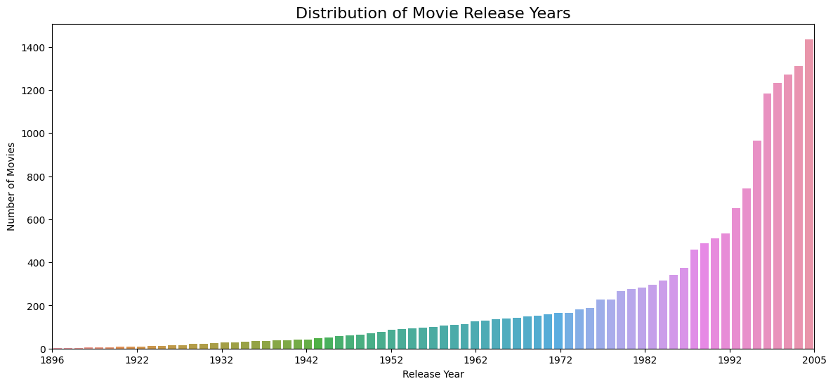
When were the movies released?
# Plot the movie release years and their counts
data = movie_titles['Year'].value_counts().sort_index()

plot_movie_years_counts(data)
Console output (1/1):
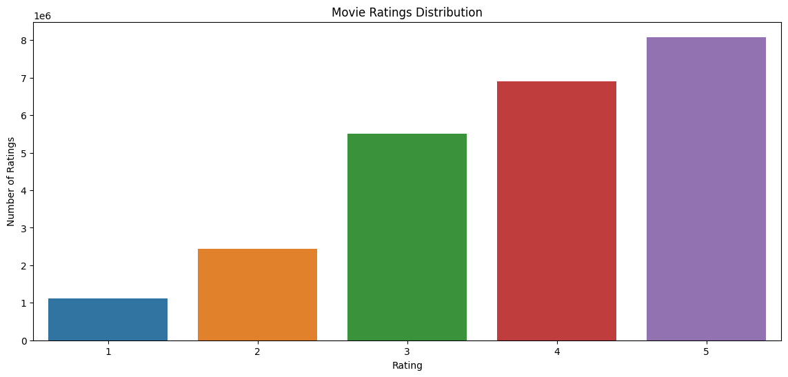
How are The Ratings Distributed?
# Plot the movie ratings distribution
data = df['Rating'].value_counts().sort_index()

plot_movie_ratings_distribution(data)
Console output (1/1):
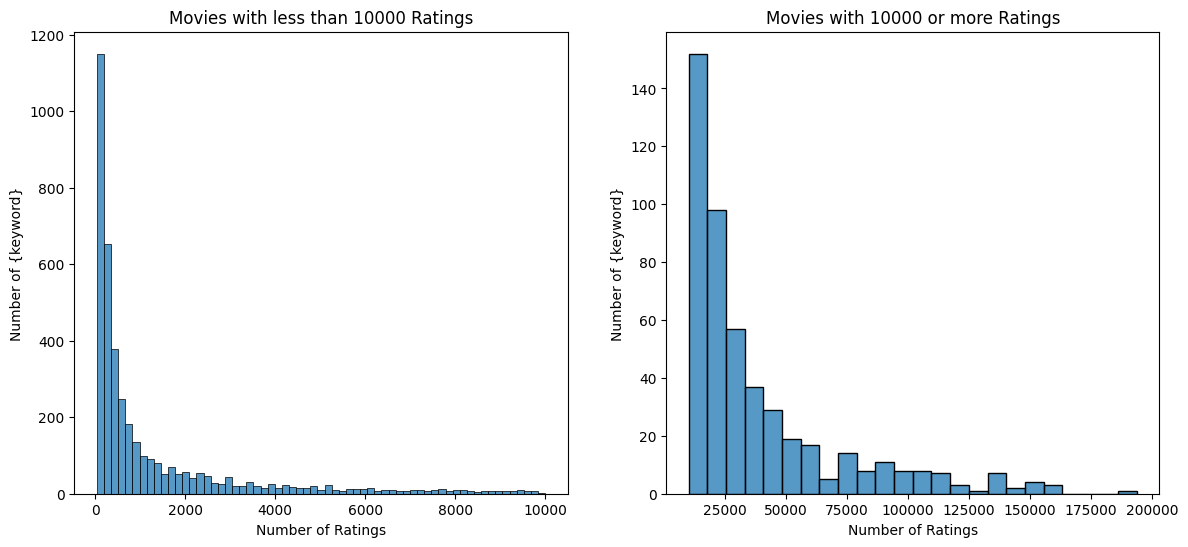
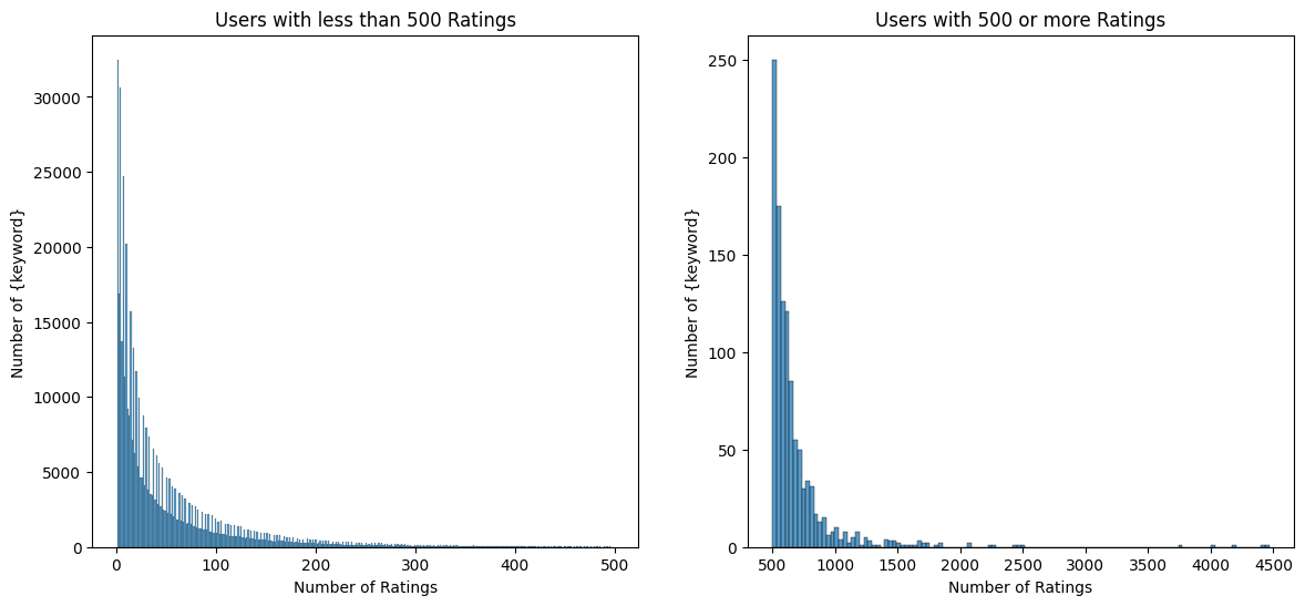
Visualize the Distribution of Number of Movie Ratings and User Rating
# Plot the movie ratings counts distribution

thresh = 10000
data = df.groupby('Movie')['Rating'].count()
plot_ratings_counts_distribution(data, thresh, 'Movies')
Console output (1/1):
thresh = 500
data = df.groupby('User')['Rating'].count()
plot_ratings_counts_distribution(data, thresh, 'Users')
Console output (1/1):
Dimensionality reduction
Filter Sparse Movies And Users
To reduce the dimensionality of the dataset I am filtering rarely rated movies and rarely rating users out.
# Filter sparse movies
min_movie_ratings = 1000
filter_movies = (df['Movie'].value_counts()>min_movie_ratings)
filter_movies = filter_movies[filter_movies].index.tolist()

# Filter sparse users
min_user_ratings = 200
filter_users = (df['User'].value_counts()>min_user_ratings)
filter_users = filter_users[filter_users].index.tolist()

# Actual filtering
df_filtered = df[(df['Movie'].isin(filter_movies)) & (df['User'].isin(filter_users))]
del filter_movies, filter_users, min_movie_ratings, min_user_ratings
print('Shape User-Ratings unfiltered:\t{}'.format(df.shape))
print('Shape User-Ratings filtered:\t{}'.format(df_filtered.shape))
Console output (1/1):
Shape User-Ratings unfiltered:	(24053764, 4)
Shape User-Ratings filtered:	(5930581, 4)
Create train and test sets
# Shuffle DataFrame
df_filtered = df_filtered.drop('Date', axis=1).sample(frac=1).reset_index(drop=True)

# Testingsize
n = 100000

# Split train- & testset
df_train = df_filtered[:-n]
df_test = df_filtered[-n:]
df_train.shape, df_test.shape
Console output (1/1):
((5830581, 3), (100000, 3))
Transformation
# Create a user-movie matrix with empty values
df_p = df_train.pivot_table(values='Rating', index='User', columns=['Movie'], fill_value=0)
print('Shape User-Movie-Matrix:\t{}'.format(df_p.shape))
Console output (1/1):
Shape User-Movie-Matrix: (20828, 1741)
Global Recommendation Systems (Mean Rating)
Computing the mean rating for all movies creates a ranking. The recommendation will be the same for all users and can be used if there is no information on the user. Variations of this approach can be separate rankings for each country/year/gender/… and to use them individually to recommend movies/items to the user.
It has to be noted that this approach is biased and favours movies with fewer ratings, since large numbers of ratings tend to be less extreme in its mean ratings.
# Compute mean rating for all movies
ratings_mean = df_p.mean(axis=0).sort_values(ascending=False).rename('Rating-Mean').to_frame()

# Compute rating frequencies for all movies
ratings_count = df_p.count(axis=0).rename('Rating-Freq').to_frame()

# Combine the aggregated dataframes
combined_df = ratings_mean.join(ratings_count).join(movie_titles)
# Join labels and predictions based on mean movie rating
predictions_df = df_test.set_index('Movie').join(ratings_mean)
predictions_df.head(5)
Console output (1/1):
.dataframe tbody tr th {
    vertical-align: top;
}

.dataframe thead th {
    text-align: right;
}
y_true = predictions_df['Rating']
y_pred = predictions_df['Rating-Mean']

rmse = np.sqrt(mean_squared_error(y_true=y_true, y_pred=y_pred))
print("The RMSE Value for the Mean Rating Recommender:", rmse)
Console output (1/1):
The RMSE Value for the Mean Rating Recommender: 2.5012923665039972
# View top ten rated movies
print(combined_df[['Name', 'Rating-Mean']].head(10))
Console output (1/1):
Name  Rating-Mean
Movie
4306                                     The Sixth Sense     4.017717
2452       Lord of the Rings: The Fellowship of the Ring     3.951988
2862                            The Silence of the Lambs     3.927982
1905   Pirates of the Caribbean: The Curse of the Bla...     3.873872
2782                                          Braveheart     3.701508
3962                           Finding Nemo (Widescreen)     3.668379
571                                      American Beauty     3.400182
798                                                 Jaws     3.331093
3938                                             Shrek 2     3.299069
1798                                       Lethal Weapon     3.270405
Global Recommendation Systems (Weighted Rating)
To tackle the problem of the unstable mean with few ratings e.g. IDMb uses a weighted rating. Many good ratings outweigh few in this algorithm.
# Number of minimum votes to be considered
m = 1000

# Mean rating for all movies
C = df_p.stack().mean()

# Mean rating for all movies separately
R = df_p.mean(axis=0).values

# Rating freqency for all movies separately
v = df_p.count().values

# Weighted formula to compute the weighted rating
weighted_score = (v/(v+m))*R + (m/(v+m))*C

# convert weighted_score into a dataframe
weighted_mean = pd.DataFrame(weighted_score, columns=['Weighted-Mean'], index=df_p.columns)

# Combine the aggregated dataframes (wighted_mean & movie_titles)
combined_df = combined_df.join(weighted_mean)
print(combined_df[['Name', 'Weighted-Mean']].head(10))
Console output (1/1):
Name  Weighted-Mean
Movie
4306                                     The Sixth Sense       3.859200
2452       Lord of the Rings: The Fellowship of the Ring       3.796482
2862                            The Silence of the Lambs       3.773576
1905   Pirates of the Caribbean: The Curse of the Bla...       3.721945
2782                                          Braveheart       3.557477
3962                           Finding Nemo (Widescreen)       3.525867
571                                      American Beauty       3.269957
798                                                 Jaws       3.204032
3938                                             Shrek 2       3.173475
1798                                       Lethal Weapon       3.146125
# Join labels and predictions based on mean movie rating
predictions_df = df_test.set_index('Movie').join(weighted_mean)

# Compute RMSE
y_true = predictions_df['Rating']
y_pred = predictions_df['Weighted-Mean'].fillna(0)

rmse = np.sqrt(mean_squared_error(y_true=y_true, y_pred=y_pred))
print("The RMSE Value for the Weighted-Mean Rating Recommender:", rmse)

print(combined_df[['Name', 'Weighted-Mean']].sort_values(by='Weighted-Mean', ascending=False).head(10))
Console output (1/1):
The RMSE Value for the Weighted-Mean Rating Recommender: 2.5190629723842495
                                                    Name  Weighted-Mean
Movie
4306                                     The Sixth Sense       3.859200
2452       Lord of the Rings: The Fellowship of the Ring       3.796482
2862                            The Silence of the Lambs       3.773576
1905   Pirates of the Caribbean: The Curse of the Bla...       3.721945
2782                                          Braveheart       3.557477
3962                           Finding Nemo (Widescreen)       3.525867
571                                      American Beauty       3.269957
798                                                 Jaws       3.204032
3938                                             Shrek 2       3.173475
1798                                       Lethal Weapon       3.146125
The variable “m” can be seen as regularizing parameter. Changing it determines how much weight is put onto the movies with many ratings. Even if there is a better ranking the RMSE decreased slightly. There is a trade-off between interpretability and predictive power.
Content Based Recommendation Systems
# Create tf-idf matrix for text comparison
tfidf = TfidfVectorizer(stop_words='english')
tfidf_matrix = tfidf.fit_transform(movie_metadata['overview'])
# Compute cosine similarity between all movie-descriptions
similarity = cosine_similarity(tfidf_matrix)
similarity_df = pd.DataFrame(similarity,
                             index=movie_metadata.index.values,
                             columns=movie_metadata.index.values)
print(similarity_df.head(2))
Console output (1/1):
Toy Story   Jumanji  Grumpier Old Men  Waiting to Exhale  \
Toy Story   1.000000  0.015385          0.000000                0.0
Jumanji     0.015385  1.000000          0.046854                0.0

           Father of the Bride Part II      Heat  Sabrina  Tom and Huck  \
Toy Story                          0.0  0.000000      0.0           0.0
Jumanji                            0.0  0.047646      0.0           0.0

           Sudden Death  GoldenEye  ...  The Final Storm  In a Heartbeat  \
Toy Story      0.000000        0.0  ...              0.0        0.023356
Jumanji        0.098488        0.0  ...              0.0        0.000000

           Bloed, Zweet en Tranen  To Be Fat Like Me  Cadet Kelly  \
Toy Story                     0.0           0.000000          0.0
Jumanji                       0.0           0.004192          0.0

           L'Homme à la tête de caoutchouc  Le locataire diabolique  \
Toy Story                         0.000000                      0.0
Jumanji                           0.014642                      0.0

           L'Homme orchestre  Maa  Robin Hood
Toy Story                0.0  0.0         0.0
Jumanji                  0.0  0.0         0.0

[2 rows x 21604 columns]
movie_list = similarity_df.columns.values

def content_movie_recommender(input_movie, similarity_database=similarity_df, movie_database_list=movie_list, top_n=10):

    """
    This function takes in a movie name and returns the top n similar movies.

    Parameters
    ----------
    input_movie : str
        The movie name for which similar movies are to be found.

    similarity_database : pandas.DataFrame
        The similarity database for all movies.

    movie_database_list : list
        The list of all movies.

    top_n : int
        The number of similar movies to be returned.

    Returns
    -------
    recommended_movies : list
        The list of top n similar movies.

    """


    # movie list
    movie_list = movie_database_list

    # get movie similarity records
    movie_sim = similarity_database[similarity_database.index == input_movie].values[0]

    # get movies sorted by similarity
    sorted_movie_ids = np.argsort(movie_sim)[::-1]

    # get recommended movie names
    recommended_movies = movie_list[sorted_movie_ids[1:top_n+1]]

    print('\n\nTop Recommended Movies for:', input_movie, 'are:-\n', recommended_movies)


sample_movies = ['Captain America', 'The Terminator', 'The Exorcist',
                 'The Hunger Games: Mockingjay - Part 1', 'The Blair Witch Project']

for movie in sample_movies:
    content_movie_recommender(movie)
Console output (1/1):
Top Recommended Movies for: Captain America are:-
 ['Iron Man & Captain America: Heroes United'
 'Captain America: The First Avenger' 'Team Thor' 'Education for Death'
 'Captain America: The Winter Soldier' '49th Parallel' 'Ultimate Avengers'
 'Philadelphia Experiment II' 'Vice Versa' 'The Lair of the White Worm']


Top Recommended Movies for: The Terminator are:-
 ['Terminator 2: Judgment Day' 'Terminator Salvation'
 'Terminator 3: Rise of the Machines' 'Silent House' 'They Wait'
 'Another World' 'Teenage Caveman' 'Appleseed Alpha' 'Respire'
 'Just Married']


Top Recommended Movies for: The Exorcist are:-
 ['Exorcist II: The Heretic' 'Domestic Disturbance' 'Damien: Omen II'
 'The Exorcist III' 'Like Sunday, Like Rain' 'People Like Us'
 'Quand on a 17 Ans' "Don't Knock Twice" 'Zero Day' 'Brick Mansions']


Top Recommended Movies for: The Hunger Games: Mockingjay - Part 1 are:-
 ['The Hunger Games: Catching Fire' 'The Hunger Games: Mockingjay - Part 2'
 'Last Train from Gun Hill' 'The Hunger Games'
 'Will Success Spoil Rock Hunter?' 'Circumstance' 'Man of Steel'
 'The Amityville Horror' 'Pregnancy Pact' 'Bananas']


Top Recommended Movies for: The Blair Witch Project are:-
 ['Book of Shadows: Blair Witch 2' 'Freakonomics' 'Le Bal des actrices'
 'Greystone Park' 'Willow Creek' 'Addio zio Tom' 'The Conspiracy'
 'A Haunted House' 'Tonight She Comes' 'Curse of the Blair Witch']