Time Series Forecasting
Time Series is a big component of our everyday lives. They are in fact used in medicine (EEG analysis), finance (Stock Prices) and electronics (Sensor Data Analysis). Many Machine Learning models have been created in order to tackle these types of tasks, two examples are ARIMA (AutoRegressive Integrated Moving Average) models and RNNs (Recurrent Neural Networks).
Data Source
For Time series analysis, we are going to deal with Stock market Analysis. This dataset is based US-based stocks daily price and volume data. Dataset taken for analysis is IBM stock market data from 2006-01-01 to 2018-01-01.
Below are the key fields in the dataset:
Date, Open, High, Low, Close, Volume, Name
import warnings
warnings.filterwarnings('ignore')

import pandas as pd
import matplotlib.pyplot as plt
import numpy as np
from pandas.plotting import lag_plot

from statsmodels.tsa.stattools import adfuller
from statsmodels.graphics.tsaplots import plot_acf, plot_pacf

from statsmodels.tsa.arima.model import ARIMA
from sklearn.metrics import mean_squared_error
EDA and Data Wrangling
df = pd.read_csv("IBM_2006-01-01_to_2018-01-01.csv.zip")
print(df.head())
Console output (1/1):
Date   Open   High    Low  Close    Volume Name
0  2006-01-03  82.45  82.55  80.81  82.06  11715200  IBM
1  2006-01-04  82.20  82.50  81.33  81.95   9840600  IBM
2  2006-01-05  81.40  82.90  81.00  82.50   7213500  IBM
3  2006-01-06  83.95  85.03  83.41  84.95   8197400  IBM
4  2006-01-09  84.10  84.25  83.38  83.73   6858200  IBM
# Cleaning up the data
df.isnull().values.any()
df = df.dropna()
df.shape
Console output (1/1):
(3019, 7)
df.index = pd.to_datetime(df['Date'])
print(df.head())
Console output (1/1):
Date   Open   High    Low  Close    Volume Name
Date
2006-01-03  2006-01-03  82.45  82.55  80.81  82.06  11715200  IBM
2006-01-04  2006-01-04  82.20  82.50  81.33  81.95   9840600  IBM
2006-01-05  2006-01-05  81.40  82.90  81.00  82.50   7213500  IBM
2006-01-06  2006-01-06  83.95  85.03  83.41  84.95   8197400  IBM
2006-01-09  2006-01-09  84.10  84.25  83.38  83.73   6858200  IBM
Visualization
fig, axes = plt.subplots(1, 3, figsize=(18, 6))

dr = df[['High', 'Low']]
dr.plot(ax=axes[0])
axes[0].set_title('IBM High-Low Returns')

dr = df[['Open', 'Close']]
dr.plot(ax=axes[1])
axes[1].set_title('IBM Open-Close Returns')

dr = df.cumsum()[['Open', 'Close']]
dr.plot(ax=axes[2])
axes[2].set_title('IBM Cumulative Open-Close Returns')

plt.show()
Console output (1/1):
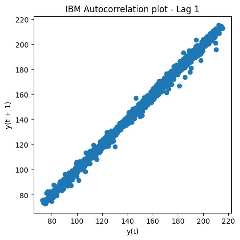
Autocorrelation plot
plt.figure(figsize=(5,5))
lag_plot(df['Open'], lag=1)
plt.title('IBM Autocorrelation plot - Lag 1')
plt.show()
Console output (1/1):
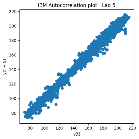
Visualize the Auto-Correlation plot for IBM Open prices with Lag 5
plt.figure(figsize=(5,5))
lag_plot(df['Open'], lag=5)
plt.title('IBM Autocorrelation plot - Lag 5')
plt.show()
Console output (1/1):
def plot_ibm_prices(train_data, test_data):
    """
    Plots the training and testing data for IBM stock prices.

    Args:
        train_data (pd.DataFrame): A DataFrame containing the training data.
        test_data (pd.DataFrame): A DataFrame containing the testing data.
    """
    fig, ax = plt.subplots(figsize=(12, 7))

    ax.set_title('IBM Prices')
    ax.set_xlabel('Dates')
    ax.set_ylabel('Prices')

    ax.plot(train_data['Open'], 'blue', label='Training Data')
    ax.plot(test_data['Open'], 'green', label='Testing Data')

    ax.legend()
    plt.show()

def plot_rolling_statistics(train_series, window=7):
    """
    Plots the rolling mean and standard deviation for a time series.

    Args:
        train_series (pd.Series): A Series containing the time series data.
        window (int): The window size for the rolling statistics.
    """
    # Determine rolling statistics
    rolmean = train_series.rolling(window).mean()
    rolstd = train_series.rolling(window).std()

    # Plot rolling statistics
    fig, ax = plt.subplots(figsize=(10, 6))
    orig = ax.plot(train_series, color='blue', label='Original')
    mean = ax.plot(rolmean, color='red', label='Rolling Mean')
    std = ax.plot(rolstd, color='black', label='Rolling Std')
    ax.legend(loc='best')
    ax.set_title('Rolling Mean & Standard Deviation')

    plt.show()

def plot_rolling_statistics_diff(train_diff, window=7):
    """
    Plots the rolling mean and standard deviation for a differenced time series.

    Args:
        train_diff (pd.Series): A Series containing the differenced time series data.
        window (int): The window size for the rolling statistics.
    """
    # Determine rolling statistics
    rolmean = train_diff.rolling(window).mean()
    rolstd = train_diff.rolling(window).std()

    # Plot rolling statistics
    fig, ax = plt.subplots(figsize=(10, 6))
    orig = ax.plot(train_diff, color='blue', label='Original')
    mean = ax.plot(rolmean, color='red', label='Rolling Mean')
    std = ax.plot(rolstd, color='black', label='Rolling Std')
    ax.legend(loc='best')
    ax.set_title('Rolling Mean & Standard Deviation on the Difference')

    plt.show()
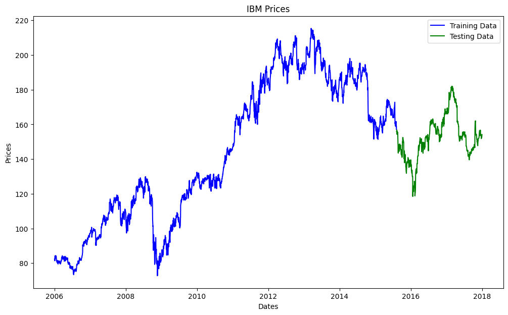
Splitting into testing and training data
train_data, test_data = df.iloc[0:int(len(df)*0.8), :], df.iloc[int(len(df)*0.8):, :]

plot_ibm_prices(train_data, test_data)
Console output (1/1):
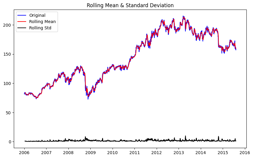
Performing ARIMA (AutoRegressive Integrated Moving Average)
window = 7
train_series = train_data['Open']

plot_rolling_statistics(train_series, window)
Console output (1/1):
Next we will calculate the Augmented Dickey-Fuller test for stationarity of a time series data train_series. The adfuller() function from the statsmodels.tsa.stattools module is used for this purpose, with the autolag parameter set to ‘AIC’ to automatically select the best lag order for the test.
dftest = adfuller(train_series, autolag='AIC')
dfoutput = pd.Series(dftest[0:4], index=['Test Statistic','p-value','#Lags Used','Number of Observations Used'])
for key,value in dftest[4].items():
    dfoutput['Critical Value (%s)'%key] = value
dfoutput
Console output (1/1):
Test Statistic                   -1.487786
p-value                           0.539545
#Lags Used                        7.000000
Number of Observations Used    2407.000000
Critical Value (1%)              -3.433070
Critical Value (5%)              -2.862742
Critical Value (10%)             -2.567410
dtype: float64
Observation:
p-value is not less than 0.05, series is not stationary.
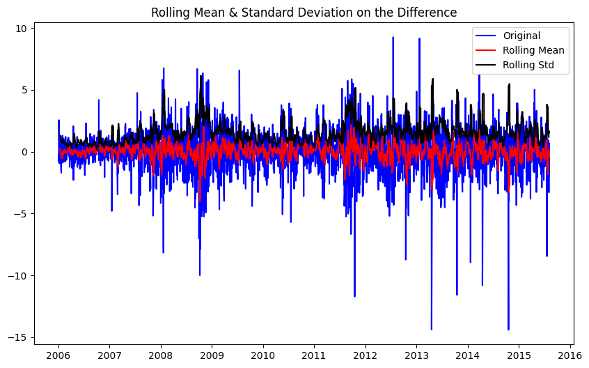
Apply a first order differencing on the training data
train_diff = train_series.diff()
train_diff = train_diff.dropna(inplace = False)
plot_rolling_statistics_diff(train_diff, window=7)
Console output (1/1):
AD-Fuller Stats for differenced train data
dftest = adfuller(train_diff, autolag='AIC')
dfoutput = pd.Series(dftest[0:4], index=['Test Statistic','p-value','#Lags Used','Number of Observations Used'])
for key,value in dftest[4].items():
    dfoutput['Critical Value (%s)'%key] = value
dfoutput
Console output (1/1):
Test Statistic                  -20.324277
p-value                           0.000000
#Lags Used                        6.000000
Number of Observations Used    2407.000000
Critical Value (1%)              -3.433070
Critical Value (5%)              -2.862742
Critical Value (10%)             -2.567410
dtype: float64
After differencing, the p-value is extremely small. Thus this series is very likely to be stationary.
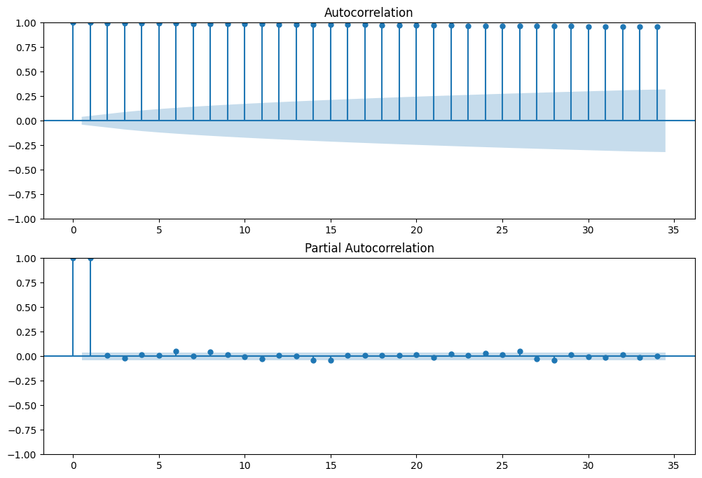
Plot ACF and PACF on the original train series
fig, ax = plt.subplots(2, 1, figsize=(12,8))
plot_acf(train_series, ax=ax[0]); #
plot_pacf(train_series, ax=ax[1])
plt.show()
Console output (1/1):
Plot ACF and PACF on the differenced train series
fig, ax = plt.subplots(2, 1, figsize=(12,8))
plot_acf(train_diff, ax=ax[0]); #
plot_pacf(train_diff, ax=ax[1])
plt.show()
Console output (1/1):
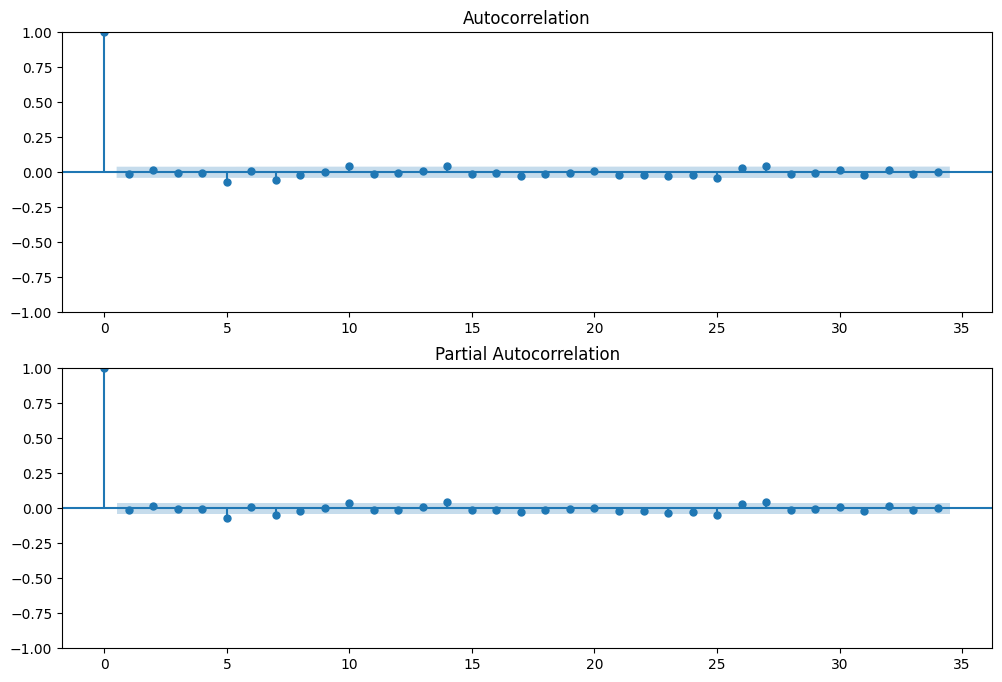
Determininig p, d, q
- p=5
- d=1
- q=0
def smape_kun(y_true, y_pred):
    """
    Computes the symmetric mean absolute percentage error (SMAPE) between two arrays.

    Args:
        y_true (np.array): An array of ground truth values.
        y_pred (np.array): An array of predicted values.

    Returns:
        float: The SMAPE between `y_true` and `y_pred`.
    """
    # Compute SMAPE
    return np.mean((np.abs(y_pred - y_true) * 200 / (np.abs(y_pred) + np.abs(y_true))))
test_series = test_data['Open']
test_diff = test_series.diff()
test_diff = test_diff.dropna(inplace = False)
%%time
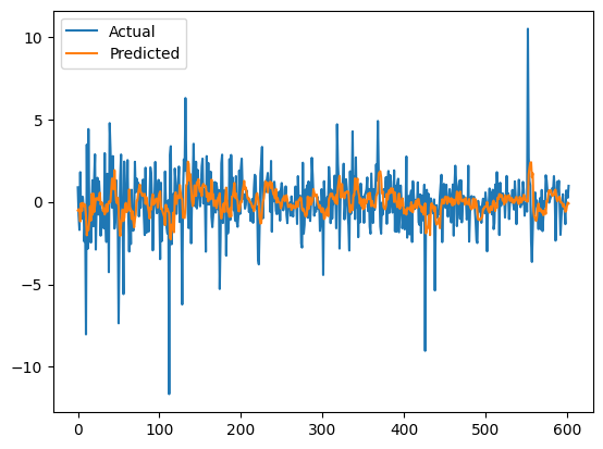
history = [x for x in train_diff]
predictions = list()
for t in range(len(test_diff)):
# initialize the model with history and right order of parameters
model = ARIMA(history, order=(5,1,0))
# fit the model
model_fit = model.fit()
# use forecast on the fitted model
output = model_fit.forecast()
yhat = output[0]
predictions.append(yhat)
obs = test_diff[t]
history.append(obs)
if t % 100 == 0:
print('Test Series Point: {}\tPredicted={}, Expected={}'.format(t, yhat, obs))
Console output (1/1):
Test Series Point: 0	Predicted=-0.5229671125021065, Expected=0.8800000000000239
Test Series Point: 100	Predicted=0.5049973042749393, Expected=-0.5100000000000193
Test Series Point: 200	Predicted=0.035878315975330644, Expected=2.0500000000000114
Test Series Point: 300	Predicted=-0.3784100169699953, Expected=-0.020000000000010232
Test Series Point: 400	Predicted=-0.7058202182006886, Expected=-0.36000000000001364
Test Series Point: 500	Predicted=-0.29631462259624564, Expected=0.5699999999999932
Test Series Point: 600	Predicted=-0.22433188016459504, Expected=0.4399999999999977
CPU times: user 2min 2s, sys: 4min 9s, total: 6min 12s
Wall time: 1min 34s
# plot actual values
plt.plot(test_diff.values, label='Actual')

# plot predicted values
plt.plot(predictions, label='Predicted')

plt.legend()
plt.show()
Console output (1/1):
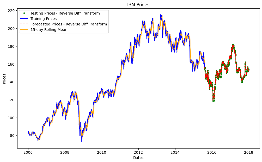
Reverse Transform the forecasted values
Since we used differencing of the first order in the series before training, we need to reverse transform the values to get meaningful price forecasts.
reverse_test_diff = np.r_[test_series.iloc[0], test_diff].cumsum()
reverse_predictions = np.r_[test_series.iloc[0], predictions].cumsum()
reverse_test_diff.shape, reverse_predictions.shape
Console output (1/1):
((604,), (604,))
Evaluate model performance
error = mean_squared_error(reverse_test_diff, reverse_predictions)
print('Testing Mean Squared Error: %.3f' % error)
error2 = smape_kun(reverse_test_diff, reverse_predictions)
print('Symmetric Mean absolute percentage error: %.3f' % error2)
Console output (1/1):
Testing Mean Squared Error: 17.604
Symmetric Mean absolute percentage error: 2.390
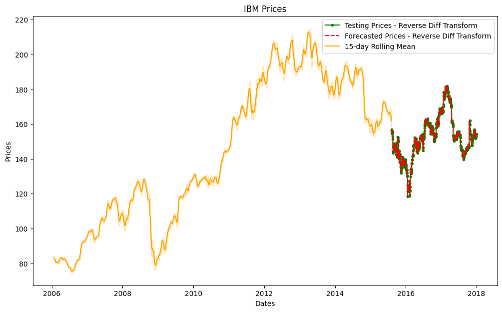
Let’s Visualize the forecast results
def plot_forecast(train_series, reverse_test_diff_series, reverse_forecast_diff_series, window=30, flag=True):
    """
    Plots the original and forecasted prices for a time series.

    Args:
        train_series (pd.Series): A Series containing the training data.
        reverse_test_diff_series (pd.Series): A Series containing the testing data, after reversing the differencing.
        reverse_forecast_diff_series (pd.Series): A Series containing the forecasted data, after reversing the differencing.
        window (int): The size of the rolling window to use for the rolling mean and standard deviation. Default is 30.
    """
    # Calculate rolling mean and standard deviation
    rolmean = train_series.rolling(window).mean()
    rolstd = train_series.rolling(window).std()

    # Plot original and forecasted prices
    fig, ax = plt.subplots(figsize=(12, 7))

    ax.plot(reverse_test_diff_series, color='green', marker='.', label='Testing Prices - Reverse Diff Transform')
    if flag:
        ax.plot(train_series, color='blue', label='Training Prices')
        ax.plot(reverse_forecast_diff_series, color='red', linestyle='--', label='Forecasted Prices - Reverse Diff Transform')
    else:
        ax.plot(reverse_test_diff_series, color='red', linestyle='--', label='Forecasted Prices - Reverse Diff Transform')
    ax.plot(rolmean, color='orange', label=f'{window}-day Rolling Mean')
    ax.fill_between(rolstd.index, rolmean-rolstd, rolmean+rolstd, alpha=0.2, color='orange')
    ax.set_title('IBM Prices')
    ax.set_xlabel('Dates')
    ax.set_ylabel('Prices')
    ax.legend()

    plt.show()
reverse_test_diff_series = pd.Series(reverse_test_diff)
reverse_test_diff_series.index = test_series.index

reverse_predictions_series = pd.Series(reverse_test_diff)
reverse_predictions_series.index = test_series.index
# Plot the forecasted prices
plot_forecast(train_series, reverse_test_diff_series, reverse_predictions_series, window=15)
Console output (1/1):
Visualize only test and forecast prices
plot_forecast(train_series, reverse_test_diff_series, reverse_predictions_series, window=15, flag=False)
Console output (1/1):